𝕁𝕋+ - How to conduct simple slope analysis and make plot with brms

Goal. In this note, we will demonstrate how to use the output from brms to make (simple slope) testings and plots.

Make data

Code

library(tidyverse)
library(brms)
library(bayestestR)
library(rstan)
library(mvtnorm)

Now we have to make a data set including 4 variables: Y, X, M, and W.

Suppose these four variables follow a multivariate-normal distribution as follows,

Let X is a treatment (binary data), and M is a response time data (lognormal).

\[\begin{equation} \begin{bmatrix} Y \\ X \\M \\W \end{bmatrix} = \text{MVN}\left( \begin{bmatrix} 0 \\0 \\ 0\\ 0 \end{bmatrix}, \begin{bmatrix} 1 & 0.1 & -0.8 & 0.8 \\ 0.1 & 1 & -0.6 & 0\\ -0.8 & -0.6 & 1 & 0.6\\ 0.8 & 0 & 0.6 & 1 \end{bmatrix} \right) \end{equation}\]

Code

set.seed(12345)
real_sigma <- matrix(c(1, 0.1, -0.8, 0.8,
                      0.1, 1, -0.6, 0,
                      -0.8, -0.6, 1, 0.6,
                      0.8, 0, 0.6, 1), nrow = 4)
real_mean <- c(0,0,0,0)

real_data <- rmvnorm(n = 1000, mean = real_mean, sigma = real_sigma)

Warning in rmvnorm(n = 1000, mean = real_mean, sigma = real_sigma): sigma is
numerically not positive semidefinite

Code

dat <- data.frame(
  ID = paste0('s', str_pad(1:1000, width = 4, side = 'left', pad = 0)),
  Y = real_data[,1],
  X = real_data[,2] > mean(real_data[,2]),
  M = exp(real_data[,3]),
  W = real_data[,4]
)

head(dat)

     ID          Y     X         M          W
1 s0001  0.3617174  TRUE 0.4790760 -0.1639895
2 s0002  0.1110080 FALSE 2.0490296  0.2046531
3 s0003  0.6187169 FALSE 2.6247616  1.4401394
4 s0004  1.0347476  TRUE 0.5084054  0.6434533
5 s0005 -1.1477318 FALSE 4.8633851  0.2686688
6 s0006  0.2802449  TRUE 0.1476185 -1.2412565

Fit Bayesian model in `brms`

Now we specify the formula as follows (in Bayesian).

\[\begin{align} \text{Likelihood.}\\ Y &\sim N(\mu_y, \sigma_y^2) \\ M &\sim \log N(\mu_m, \sigma_m^2) \\ \mu_y &= \beta_{01} + \beta_x X + \beta_m M + \beta_w W + \beta _{mw}M \cdot W \\ \mu_m &= \beta_{02} + \beta_x X \\ \\ \text{Priors.}\\ \sigma_y^2, \sigma_m^2 & \sim \text{Exp}(1) \\ \beta_{01}, ..., \beta _{x} &\sim N(0,5) \end{align}\]

Code

bf1 <- bf(Y~X+M+W+M*W, family = gaussian())
bf2 <- bf(M~X, family = lognormal())
priors <- prior(normal(0,5), class = b, resp = Y) + 
  prior(normal(0,5), class = b, resp = M) + 
  prior(exponential(1), class = sigma, resp = Y) +
  prior(exponential(1), class = sigma, resp = M) 



fit <- brm(
  bf1+bf2+set_rescor(FALSE), 
  data = dat,
  cores = 4
)

Compiling Stan program...

Start sampling

Code

print(fit, digits = 3)

 Family: MV(gaussian, lognormal) 
  Links: mu = identity; sigma = identity
         mu = identity; sigma = identity 
Formula: Y ~ X + M + W + M * W 
         M ~ X 
   Data: dat (Number of observations: 1000) 
  Draws: 4 chains, each with iter = 2000; warmup = 1000; thin = 1;
         total post-warmup draws = 4000

Regression Coefficients:
            Estimate Est.Error l-95% CI u-95% CI  Rhat Bulk_ESS Tail_ESS
Y_Intercept    0.648     0.035    0.580    0.716 1.001     4338     3242
M_Intercept    0.490     0.043    0.407    0.574 1.002     4917     3090
Y_XTRUE       -0.164     0.039   -0.241   -0.086 1.000     4874     3349
Y_M           -0.366     0.010   -0.386   -0.346 1.001     3476     3265
Y_W            0.604     0.020    0.565    0.641 1.000     4427     3384
Y_M:W          0.100     0.006    0.088    0.112 1.000     2928     2864
M_XTRUE       -0.856     0.059   -0.970   -0.742 1.001     5208     2953

Further Distributional Parameters:
        Estimate Est.Error l-95% CI u-95% CI  Rhat Bulk_ESS Tail_ESS
sigma_Y    0.570     0.013    0.544    0.597 1.000     5277     2537
sigma_M    0.962     0.021    0.921    1.005 1.002     5424     2974

Draws were sampled using sampling(NUTS). For each parameter, Bulk_ESS
and Tail_ESS are effective sample size measures, and Rhat is the potential
scale reduction factor on split chains (at convergence, Rhat = 1).

Bayesian testing

Code

fit |> 
  describe_posterior(
    effects = "all",
    component = "all",
    #test = c("p_direction", "p_significance"),
    centrality = "all"
  )

Warning: Multivariate response models are not yet supported for tests `rope` and
  `p_rope`.

Summary of Posterior Distribution M

Parameter   | Response | Median |  Mean |   MAP |         95% CI |   pd |  Rhat |     ESS
-----------------------------------------------------------------------------------------
(Intercept) |        M |   0.49 |  0.49 |  0.49 | [ 0.41,  0.57] | 100% | 1.000 | 4898.00
XTRUE       |        M |  -0.85 | -0.86 | -0.85 | [-0.97, -0.74] | 100% | 0.999 | 5258.00

# Fixed effects sigma M

Parameter | Response | Median | Mean |  MAP |         95% CI |   pd |  Rhat |     ESS
-------------------------------------------------------------------------------------
sigma     |        M |   0.96 | 0.96 | 0.96 | [ 0.92,  1.00] | 100% | 1.000 | 5345.00

# Fixed effects Y

Parameter   | Response | Median |  Mean |   MAP |         95% CI |   pd |  Rhat |     ESS
-----------------------------------------------------------------------------------------
(Intercept) |        Y |   0.65 |  0.65 |  0.65 | [ 0.58,  0.72] | 100% | 1.000 | 4325.00
XTRUE       |        Y |  -0.16 | -0.16 | -0.16 | [-0.24, -0.09] | 100% | 1.000 | 4867.00
M           |        Y |  -0.37 | -0.37 | -0.36 | [-0.39, -0.35] | 100% | 1.001 | 3499.00
W           |        Y |   0.60 |  0.60 |  0.60 | [ 0.56,  0.64] | 100% | 1.000 | 4384.00
M:W         |        Y |   0.10 |  0.10 |  0.10 | [ 0.09,  0.11] | 100% | 1.000 | 2908.00

# Fixed effects sigma Y

Parameter | Response | Median | Mean |  MAP |         95% CI |   pd |  Rhat |     ESS
-------------------------------------------------------------------------------------
sigma     |        Y |   0.57 | 0.57 | 0.57 | [ 0.54,  0.60] | 100% | 1.000 | 5226.00

The function hypothesis() can be used to test specific parameter.

Code

fit_hypo <- hypothesis(
  fit, 
  class = 'b',
  alpha = .05,
  hypothesis = 
  c(
    Low = "Y_M - Y_M:W = 0",
    Medium = "Y_M = 0",
    High = "Y_M + Y_M:W = 0")
  ) 
fit_hypo

Hypothesis Tests for class b:
  Hypothesis Estimate Est.Error CI.Lower CI.Upper Evid.Ratio Post.Prob Star
1        Low    -0.47      0.02    -0.50    -0.44         NA        NA    *
2     Medium    -0.37      0.01    -0.39    -0.35         NA        NA    *
3       High    -0.27      0.01    -0.28    -0.25         NA        NA    *
---
'CI': 90%-CI for one-sided and 95%-CI for two-sided hypotheses.
'*': For one-sided hypotheses, the posterior probability exceeds 95%;
for two-sided hypotheses, the value tested against lies outside the 95%-CI.
Posterior probabilities of point hypotheses assume equal prior probabilities.

Make plots

Code

## plotting ----
cond_plot <- conditional_effects(fit)

Code

cond_plot$`Y.Y_M:W` |>
  ggplot(aes(x = M, y = Y), ) +
  
  geom_ribbon(aes(x = effect1__, y = estimate__, linetype = effect2__,
                  ymin = lower__, ymax = upper__, fill = factor(effect2__)), alpha = 0.5) +
  geom_line(aes(x = effect1__, y = estimate__, linetype = effect2__)) +
  scale_fill_manual(name = 'W effects',
                    values = c("coral4", "coral3", "coral2"),
                    labels = c("High \n(Mean+1SD)", "Average \n(Mean)", "Low \n(Mean-1SD)"),
                    ) +
  scale_linetype_manual(name = 'W effects',
                        values = c("solid", "dotted", "dashed"),
                        labels = c("High \n(Mean+1SD)", "Average \n(Mean)", "Low \n(Mean-1SD)")) +
  labs(x = "the M", 
       y = "the Y") +
  ggtitle('M * W') +
  annotate("text", x=10, y=-8, label= "Low \n b=-0.47, [-0.49, -0.44]") +
  annotate("text", x=25, y=-7, label= "Average \n b=-0.37, [-0.38, -0.35]") +
  annotate("text", x=20, y=0, label= "High \n b=-0.27, [-0.28, -0.25]") +
  
  theme_minimal(base_size = 16)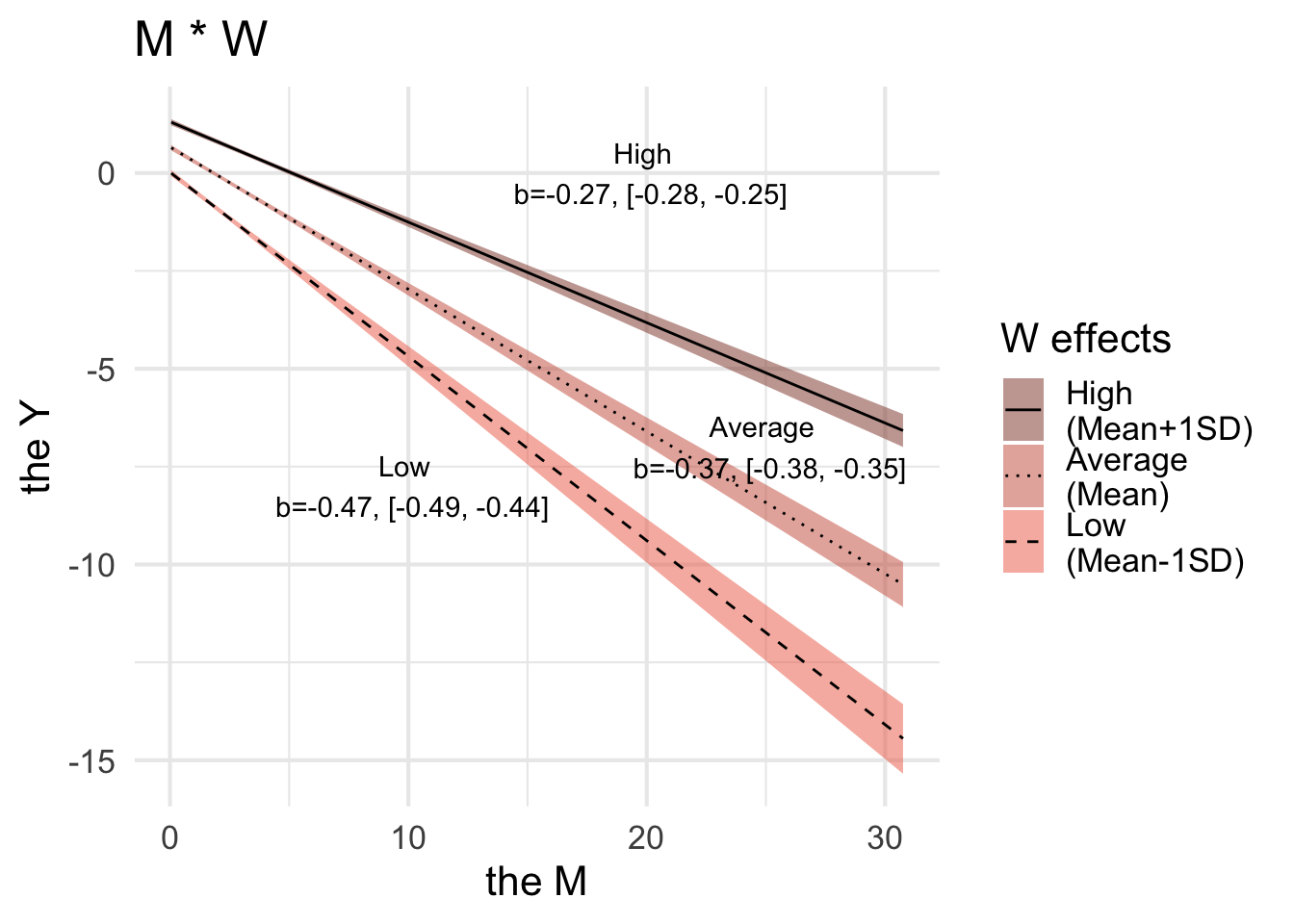

Citation

BibTeX citation:

@online{tsai2024,
  author = {Tsai, JW},
  title = {How to Conduct Simple Slope Analysis and Make Plot with
    `Brms`},
  date = {2024-03-22},
  langid = {en}
}

For attribution, please cite this work as:

Tsai, J. (2024, March 22). How to conduct simple slope analysis and make plot with `brms`.

Make data

Fit Bayesian model in brms

Bayesian testing

Make plots

Citation

Fit Bayesian model in `brms`